- Example 1: First Steps
- Example 2: Terrain
- Example 3: Mesh 2D (Smile)
- Example 4: Loop and Array
- Example 5: 1D Function (Contrast Curve)
- Example 6: 2D Function (Rocky Noise)
- Example 7: 3D Function (Seamless Noise)
- Example 8: Generative AI with Controlnet
Example 1: First Steps
Figure Ex 1.1 shows a node graph that generates an eroded terrain.
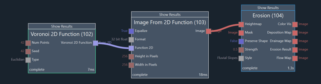
Node (102) is used to create a 2D function in the shape of Voronoi noise. This function is converted to an image using node (103). The image is used as the input of an Erosion node (104). The eroded heightmap is available as the Erosion Result output. Figure Ex 1.2 shows the result of the erosion node.
Example 2: Terrain
Figure Ex 2.1 shows a graph that generates a terrain as well as a terrain texture.
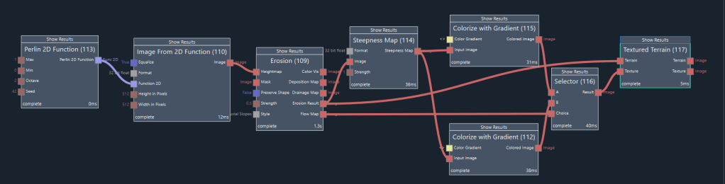
Node (113) generates a 2D function in the shape of Perlin noise. Node (110) converts this function to an image. This image is the input for the Erosion node (109). The Erosion Result output represents the eroded heightmap. It is the input for node (114), which generates a steepness map of this terrain. Nodes (115) and (112) each create a color image based on the steepness. The output of (115) will be used as the texture for those parts of the terrain where hydraulic erosion transports sediment downhill (the flow areas of the terrain). The output of (112) will be the texture for the remaining terrain. Both nodes (115) and (112) create a color image from a given gradient. The gradient can be edited by left-clicking on the node and then clicking on the button Select Scale in the top-right corner of the UI. Figure Ex 2.2 shows the gradient of node (112) and figure Ex 2.3 shows the gradient of node (115) in the gradient editor.
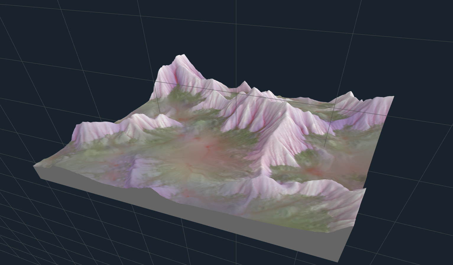
Node (116) is used to select between the two color images depending on the strength of the erosion flow, yielding the final terrain texture. Node (117) is used to visualize the terrain with the texture. Figure Ex 2.4 shows the result of node (117), the textured terrain.
Example 3: Mesh 2D (Smile)
Figure Ex 3.1 shows a node graph that creates a mesh in the shape of a smiley and renders it to an image.
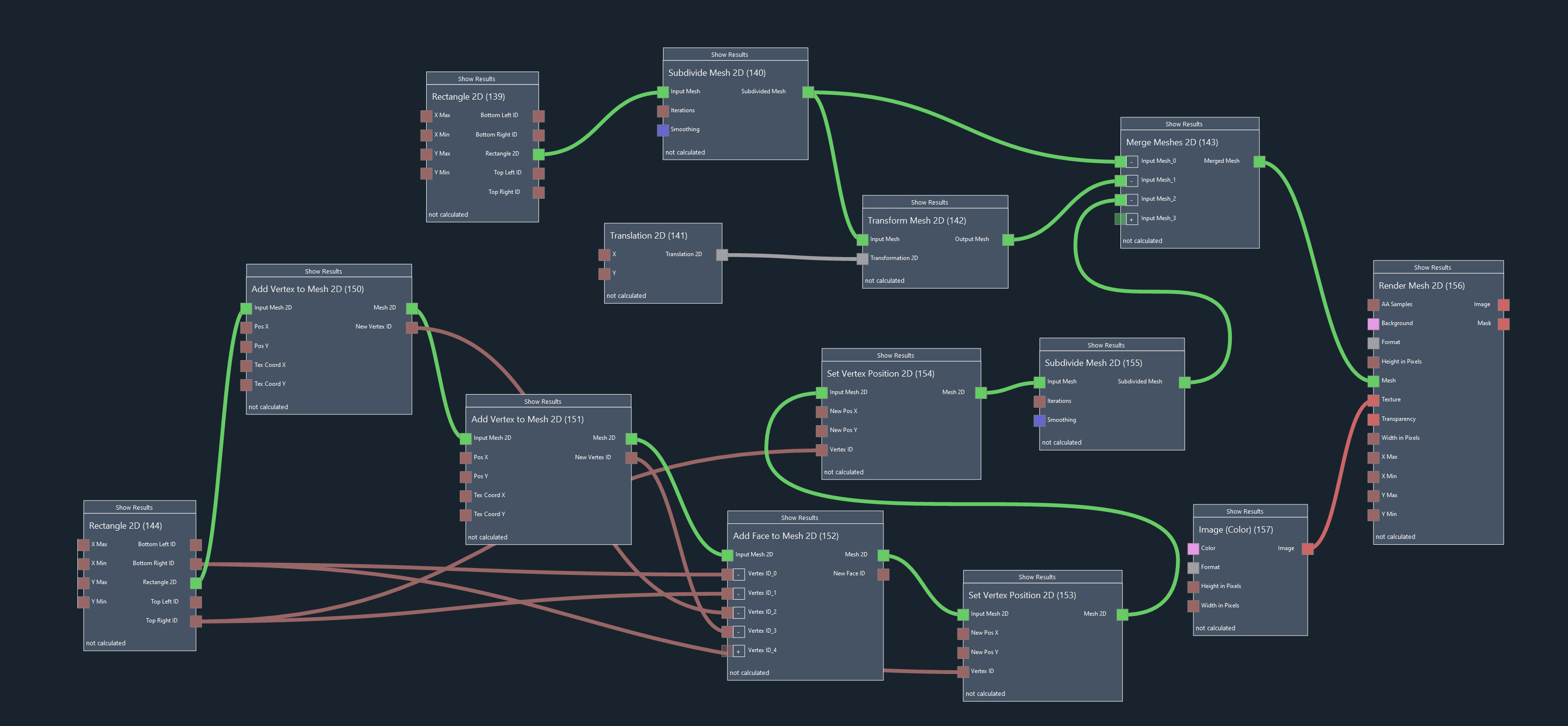
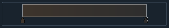
Node (144) creates a 2D mesh in the shape of a rectangle from 0.0 to 1.0 in x-direction and from -1.0 to -0.4 in y-direction. The mouth of the smiley will be generated from this rectangle with two additional points. To add two points (vertices) to the right of the original rectangle mesh, nodes (150) and (151) are used according to figure Ex 3.1. Node (150) adds a point at position (2.0, -0.4) to the top right, and node (151) adds a point at position (2.0, -1.0) to the bottom right. The two new points are still unconnected to the rest of the mesh. Node (152) connects the two rightmost points of the original rectangle with the two new points by adding a so-called “face”, a surface between four (in this case) points. This node (152) takes the mesh as input, as well as the IDs of the vertices (points) that we want to connect with a face. We now have a rectangular strip mesh that consists of 6 points (vertices). In order to bend this strip into the shape of a smiling mouth, we move the two center vertices down using nodes (153) and (154). Finally, node (155) is used to subdivide and smoothen the mouth mesh.
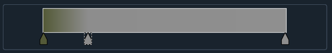
A rectangle mesh is also used as the starting point for the smiley’s eyes. Node (139) creates the rectangle and node (140) subdivides it and smoothes it into a round shape. The output of node (140) is the left eye of the smiley face. Node (141) creates a translation and node (142) applies the translation to the eye mesh, translating it in X to the right to create the right eye.
The three 2D meshes (mouth and eyes) are merged into one 2D mesh using node (143). Node (156) renders the mesh with a black texture (from node 155) onto a yellow background color. The output Image of node (156) is shown in figure Ex 3.2

Example 4: Loop and Array
Figure Ex 4.1 shows a node graph that calculates the sum of all squares between 1 and 100 (1*1 + 2*2 + … + 100 * 100) using a Loop to Array node (135).
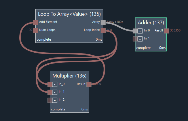
Parameter Num Loops is set to 100, so the Loop Index output will start at one and then be incremented 99 times for a final value of 100. Everytime that the Loop Index output of node (135) is reset, the following node (136) is reset and re-executed. This node (136) multiplies the Loop Index value with itself. The output Result of node (136) is “looped back” to the Add Element input of the Loop to Array node (135), so that an array is created that consists of all the result values of each loop iteration. After 100 loop iterations are calculated, the Array output of node (135) will contain all squares between 1 and 100. This array is used as the input for an Adder node (137) which yields the expected final result of 338350.
Example 5: 1D Function (Contrast Curve)
Image Ex 5.1 shows a node graph that manipulates the brightness of an image using a 1D function. A 1D function maps a scalar input value X to a scalar output value Y according to Y = F(X). An f-curve is a type of 1D function that can be edited manually in the curve editor window.
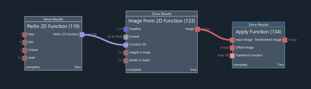
Node (119) creates Perlin Noise (a 2D function) and node (133) generates an image from this noise function. Node (134) is used to generate and apply a 1D function to the image. To edit the function, select node (134) and then click on the Adjust Function button in the parameter editor. Figure 5.2 shows the function editor window.
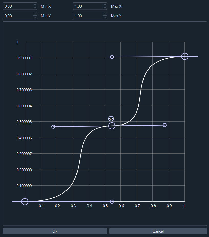
New control points can be added to the function by clicking on the line of the curve. The range in X and Y can be set in the controls above the curve editor. The result of node (134) corresponds to the Perlin noise image with manipulated brightness/ contrast curve.
Example 6: 2D Function (Rocky Noise)
Figure Ex. 6.1 shows a node graph that generates a 2D function in the shape of rocky noise. A 2D function maps a 2D vector (X, Y) input to a single scalar output value Z.
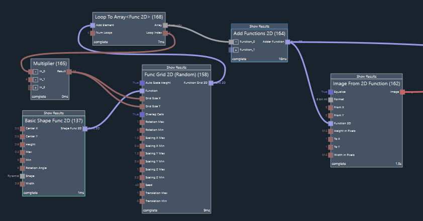
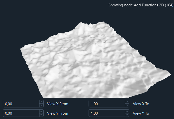
Node (137) creates a 2D function in the shape of a pyramid. This shape is repeated many times on a randomized grid using node (158). The parameter inputs of this node (158) are set so that the shape is randomly varied for each instance of the grid. Node (168) creates a loop to repeat the execution of nodes (165) and (158) four times. Each iteration will yield a 2D function in the shape of the pyramid-grid. The size of the grid is set to the Loop Index multiplied by four using node (165). The results of each iteration are combined to an array of 2D functions by node (168). All four functions in the array (the grid functions with four different grid-sizes) are summed up by node (164) to yield a 2D function in the shape of very simple rocky noise. Figure Ex 6.2 shows the result in the 2D function viewer.
Example 7: 3D Function (Seamless Noise)
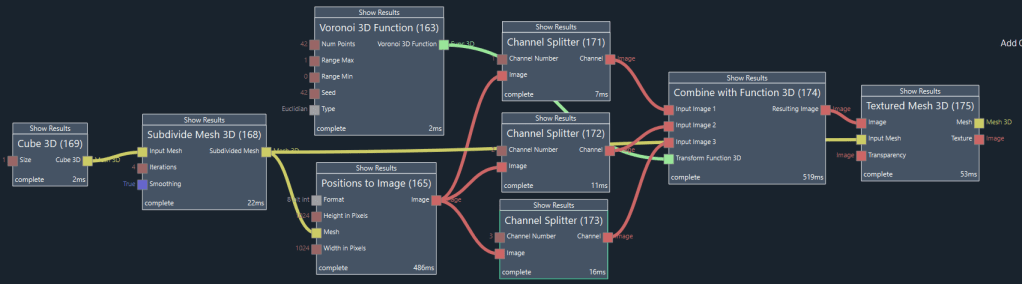
Figure Ex 7.1 shows a node graph that uses a 3D function to sample 3D noise to a texture that is seamlessly mapped on a mesh.
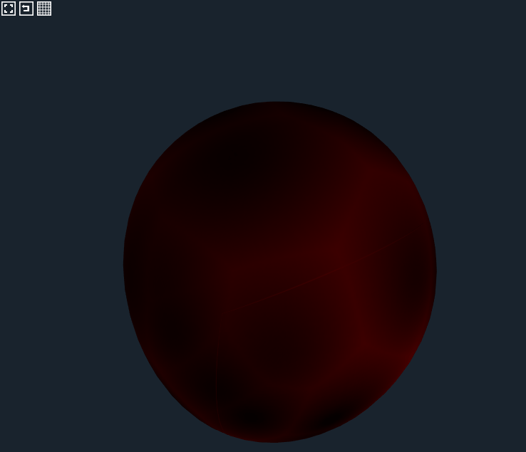
A 3D function maps a 3D vector (X, Y, Z) input to a single scalar output value W. 3D meshes are usually textured using an image and texture coordinates that map the image to the points (vertices) of the mesh. If the image contains typical noise that is generated in 2D, then the value of the noise will be different on each side of a texture seam, resulting in visible discontinuity. In this example, a 3D noise function is sampled at each position on the mesh surface. There is no discontinuity in the resulting noise texture on the mesh, as shown in figure Ex 7.2.
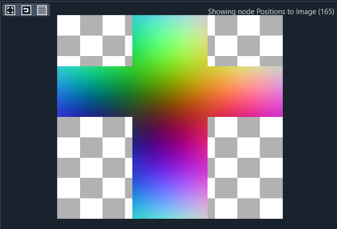
Node (169) creates a cube mesh and node (168) subdivides this mesh to create a spherical mesh shape. Node (165) maps the 3D positions of the mesh to an image according to figure Ex 7.3. Each pixel of the image represents the position on the surface of the mesh at the location of that texture coordinate. The red, green, and blue values of the pixel represent the x, y, and z value of the position on the mesh surface. These three channels are separated from the image using nodes (171), (172), and (173).
Node (163) generates a 3D Voronoi noise function. Node (174) samples this noise function at the x/y/z positions given by the outputs of nodes (171), (172), and (173), resulting in the image shown in figure Ex 7.4.

This image looks similar to regular 2D Voronoi noise, but it is slightly stretched and it is continuous across the texture seams for our mesh. Node (175) visualizes the textured mesh with the seamless noise texture applied according to figure Ex 7.2.
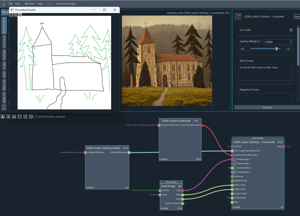
Example 8: Generative AI with Controlnet
ControlNets allow you to guide the composition of an image using structural information such as sketches, edges, or depth maps. In this example, you will turn a simple sketch into a detailed image using SDXL‑turbo and ControlNet Union, which automatically detects the type of guiding image.
- Add a Load Image node to the workspace.
- Load your guiding image — in this example, a sketch of a church with conifer trees.
- Add the node (SDXL‑turbo) Txt2Img Model.
- This loads the SDXL‑turbo model.
- Add the node (SDXL‑turbo) ControlNet Union.
- Connect the Image output of the Load Image node to the Guiding Image input of the ControlNet Union node.
- ControlNet Union automatically analyzes the sketch and selects the appropriate conditioning mode.
- Add the node (SDXL‑turbo) Txt2Img + ControlNet.
- Connect the Model output of the Txt2Img Model node to the Model input.
- Connect the ControlNet Union output to the ControlNet input.
- Enter a text prompt such as “A church with some conifer trees.”
- Set the Guiding Weight (e.g., 0.9) to control how strongly the sketch influences the final image.
- Press Execute.
- When processing is complete, click Show Result to view the generated image.
This workflow is ideal for turning rough sketches or layout drawings into fully rendered images while maintaining control over the overall structure.