- Quick Start
- The Procedural Studio GUI
- Working with Images
- Local Generative AI
- Working with Meshes
- Working with Functions
- Heightmap Generation
- Subgraphs and External Ports
- Conditional Flow Control
- Recursive Graphs
- Loops and Arrays
- Managing Graphs and Spaces
Quick Start
In the Node-Selector window (in the top left corner of the UI), select the tab Functional and scroll down to the node Perlin 2D function. Click on this node and drag it to the Editor-Area in the bottom half of the UI. Congratulations, you just created your first node-graph.
Next, select the tab Image in the Node-Selector window and add the node Image from 2D function into the Editor-Area, to the right of the node Perlin 2D function. To connect the two nodes, left-click on the output Perlin 2D function and drag to the input Function 2D.
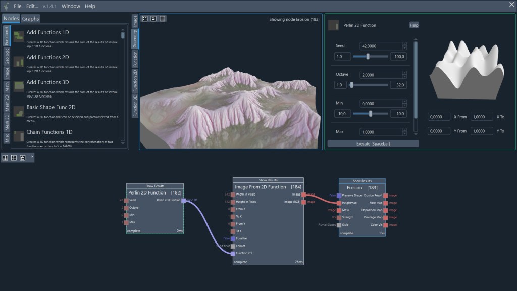
As a last node, add Erosion from the tab Geologic. Connect the output Image from the node Image from 2D function to the input Heightmap of the Erosion node. The node graph is now complete.
To execute and view the results, click on the Execute-button on the right side in the top part of the UI and wait for a few seconds while Procedural Studio calculates your graph. Click on the Show Results button on the node Erosion to view the resulting heightmap in the 3D viewer.
The Procedural Studio GUI
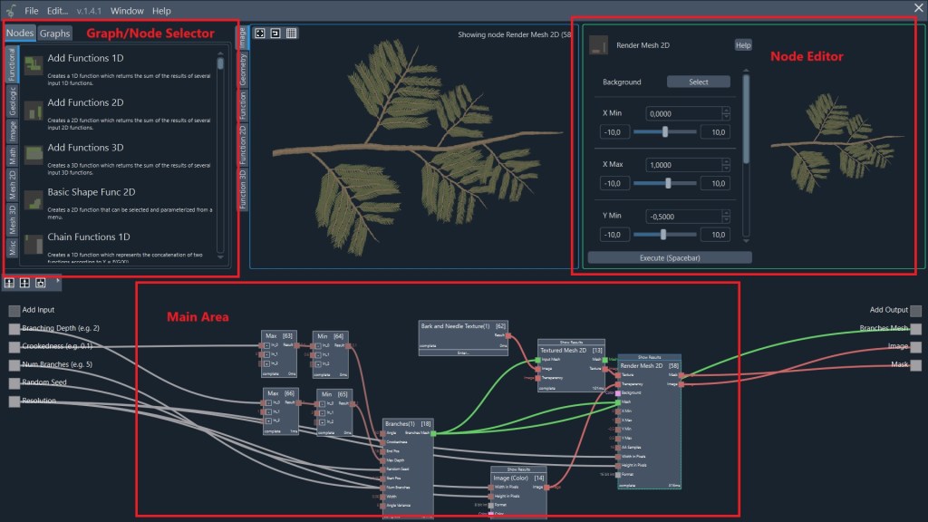
The Graph/Node-Selector window in the top left corner of the UI shows all available nodes in the top tab “Nodes”. Available graphs and spaces are shown under the top tab “Graphs”. The graphs and spaces in the tab My Box can be edited. The graphs from all other tabs (Node Boxes) can be dragged into the main area to create copies in your own workspace (My Box). Chapter “Managing Graphs and Spaces” explains how to manage graphs and workspaces in more detail.
Nodes are the basic building blocks for node graphs. These nodes can be dragged to the main area. Connect these nodes to create node-graphs that generate and manipulate images, meshes, or other assets.
The Viewer-Area window shows the output of the selected node when the graph has been calculated. Click on the button Show Results of a node after executing the graph to select the node, and the Viewer will automatically show a combination of the result outputs. Different tabs are used for the visualization of meshes, functions, or images.
The Node-Editor Area in the top right of the UI is used to set open input parameters of the currently selected node. Left-Click on a node to show the open input parameters that can be edited in the Node-Editor window. Editable parameters include numbers, colors, 1D-Functions as well as some other data types.
Finally, the main area in the bottom half of the UI shows the graph editor. Use the right mouse button to move the view and the mouse wheel to zoom. Left-clicking on a node selects the node. You can move the selected node by dragging. Use the left mouse button to rectangle-select several nodes. Connect nodes by left-clicking on an output port and dragging to an input with a green highlight. The buttons in the top left corner of the Graph-Editor are used to navigate the hierarchy and to create subgraphs from the current selection. When a subgraph is edited, the left and right side of the Graph-Editor are used to add new external ports. More information on the management of graphs and subgraphs can be found in the section “Managing Graphs and Spaces”.
Working with Images
Images in procedural studio are available with different pixel formats and different dimensions. The pixel format can be 8 bit integer, 16 bit integer, or 32 bit floating point. The desired format can usually be selected as an open input parameter for any node that generates image data. The dimensions of an image are specified by the width (the number of columns or the size of the image in x-direction), the height (the number of rows or the size of the image in y-direction), and the number of channels. Grayscale images have one single channel, color images usually have three channels in Procedural Studio. Transparency is usually stored in a separate image instead of a fourth alpha channel. However, images can have an arbitrary number of channels that can be used as desired.
To generate a color image, use the node Color Image and specify the color using the color editor from the Node-Editor. Procedural Studio provides a number of nodes used for filtering, resizing, combining, or transforming images. Most of these nodes are located in the Image tab.
Images can be loaded and saved to file using Load Image and Save Image nodes. Note that no data is saved or loaded until the graph is executed.
Local Generative AI
Generative AI in Procedural Studio enables you to create images from text descriptions, reference images, and other inputs. The workflow typically involves two steps:
- Load an AI Model using a dedicated Model node
- Generate an image using a corresponding generation node (e.g., Txt2Img)
Additional nodes allow you to refine the composition, blend AI‑generated content with classical image‑processing techniques, or build more advanced pipelines.
Generative AI requires substantial memory and compute resources. For best performance—especially when using CUDA acceleration—a modern NVIDIA GPU with a large amount of VRAM is strongly recommended.
Procedural Studio includes three publicly available Stable Diffusion models that power most generative AI nodes: - SDXL‑turbo – compact, fast, and ideal for quick iterations
- SD‑3.5‑Large‑turbo – similar memory requirements to SD‑3.5‑Large, but faster generation due to fewer inference steps
- SD‑3.5‑Large – the most capable model, with the highest overall generation quality
Each model supports a different feature set and has distinct performance characteristics.
First Steps: Your First Txt2Img Generation
- Open the Generative AI tab in the node library.
- If the tab is missing, ensure that the Generative AI plugin (free DLC) is installed and fully downloaded.
- You may need to restart Steam for updates to apply.
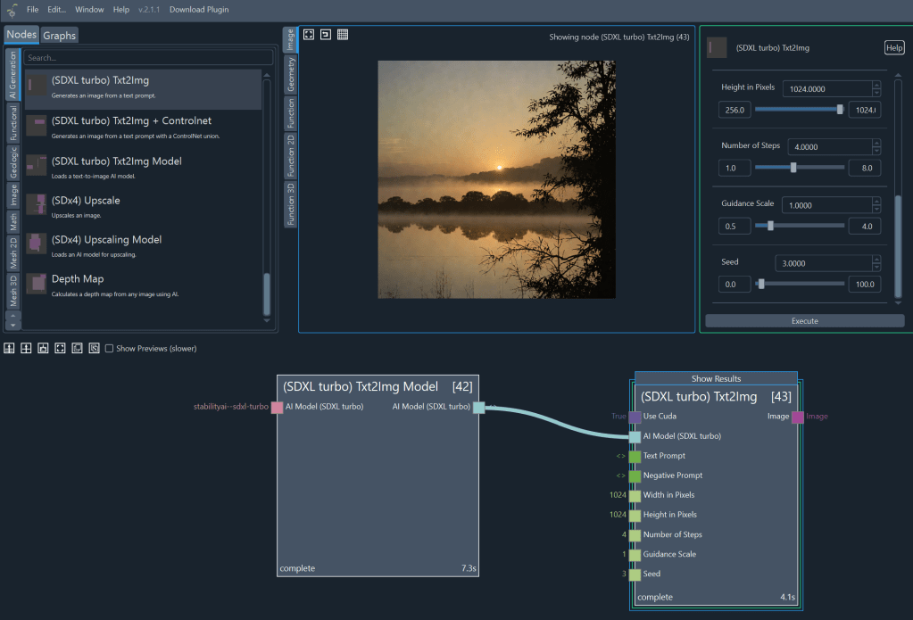
- Drag the node (SDXL‑turbo) Txt2Img Model into the main workspace.
- This node loads the SDXL‑turbo model, which is optimized for speed and low memory usage.
- Next, locate the node (SDXL‑turbo) Txt2Img and drag it into the workspace near the model node.
- Connect the model output to the model input of the Txt2Img node.
- Only one input will accept this connection.
- Press Execute.
- Depending on your hardware, generation may take anywhere from a few seconds to a few minutes.
- Once the process completes, click Show Result on the Txt2Img node to view the generated image.
- If you kept the default prompt, you should see an image of a lake.
Procedural Studio also includes a range of advanced generative AI techniques, all applied through similar model‑and‑inference workflows. These methods allow you to guide the generation process more precisely or combine AI with classical image processing:
Additional Generative AI Techniques
Upscaling
Enhances resolution and detail, allowing you to turn fast, low‑resolution drafts into high‑quality final images. Like inpainting and outpainting, upscaling relies on older Stable Diffusion models and may not match the fidelity of the newer model families.
These techniques work across models of different sizes and performance characteristics. For practical demonstrations and ready‑to‑use node graphs, refer to the Examples chapter.
Image‑to‑Image (Img2Img)
Transforms an existing image while preserving its underlying structure. Useful for style transfers, variations, or turning rough sketches into detailed results.
ControlNets
Provide explicit structural guidance—such as depth maps, edge maps, poses, or segmentation—to ensure the generated image follows a specific composition. This gives you strong control over layout while still allowing creative freedom in style and detail.
LoRAs (Low‑Rank Adaptations)
Lightweight model extensions that specialize the base model toward particular styles, subjects, or aesthetics. LoRAs expand capabilities without loading a full additional model, making them efficient and flexible.
Inpainting and Outpainting
Inpainting modifies or replaces selected regions of an image, while outpainting extends an image beyond its original borders. Both techniques are based on earlier Stable Diffusion models, so fidelity may differ from results produced by the SDXL‑turbo and SD‑3.5 model families.
Working with Meshes
Procedural Studio can be used to generate and manipulate geometry in the form of 2D Meshes and 3D Meshes. Meshes can be loaded and saved using Load Mesh and Save Mesh nodes. Note that no data is saved or loaded until the graph is executed.
To create a 3D mesh, use a generator node such as Grid 3D in the tab Mesh 3D. In this case, a 3D Mesh in the shape of a grid will be available at the output of the node. For a 2D Mesh, use a generator node such as Grid 2D.
All meshes in Procedural Studio have texture coordinates. Texture coordinates are used to specify how a texture image is mapped to the mesh surface. Texture coordinates are usually generated automatically, but they can be modified by using nodes such as Transform Tex Coords 3D. This node will modify the texture coordinates of a 3D Mesh by applying a transformation matrix (a transform 3D, which can be generated using nodes from the Math tab).
Meshes can be filtered, decimated, or subdivided. In the case of 2D Meshes, the topology of the mesh can also be manipulated by explicitly adding new vertices or faces.
Working with Functions
A mathematical function can be an input or an output of a node. It specifies how an input value or an array of input values is mapped to a single output value. Functions can be used, for example, to adjust the grayscale values of an image according to a specific curve. As another example, they can also be used to transform the vertices of a mesh along the normal direction according to a noise pattern. Different function objects can be combined or concatenated in many ways to produce more complex function objects.
A 1D function maps a single input value to an output value according to Y = F(X), where X is the input value and Y is the output value. There are many ways to generate such a 1D function object. For example, the Math Func 1D node generates a 1D function object that can be mathematically specified from a list of options. As another example, the Voronoi 1D node will generate a 1D function in the shape of so called “Voronoi” noise.
An F-Curve is a type of 1D function that can be edited graphically using the function editor. When a 1D function parameter is left as an open input of a node, that input 1D function object can usually be edited as an F-Curve by clicking on the Adjust Function button in the Node Editor.
A 2D function maps an array of two input values to a single output value according to Z = F(X, Y), where X and Y are the input values any Z is the output value. Similarly, a 3D function maps an array of three input values to a single output value according to W = F(X, Y, Z), where X, Y, and Z are the input values and W is the output value. Functions are a very powerful tool that is best understood by working through the Examples.
Heightmap Generation
Heightmap processing is one of the main use cases of Procedural Studio. Generate heightmaps with any shape and use geological simulation such as hydraulic erosion to simulate natural processes for more realistic looking terrain features.
Any grayscale image (which usually has one channel) can be used as a heightmap. Use the node Textured Terrain from the Geologic tab to create a heightmap visualization of any image. It is recommended to use a pixel format of 16 bit integer or 32 bit float, because 8 bit images lead to visible quantization errors (steps) in the output terrain.
Note that the geological simulation nodes such as Erosion have additional outputs beside the erosion result. These additional outputs like the flow map can be used (along with other maps such as steepness or curvature) to create terrain textures.
Subgraphs and External Ports
Nodes can be grouped into subgraphs to be used similar to single nodes. To create a subgraph, multi-select several nodes by left-clicking and dragging a selection rectangle. Press the third symbol in the top-left corner of the Graph-Editor (tooltip “Subgraph from Selection”) and enter a name for the subgraph. The subgraph will be created and placed into the graph at the position where the selected nodes were located. If the selected group of nodes was connected to other nodes, some inputs and outputs will automatically be generated for the subgraph.
To modify the new subgraph, click on the button Enter… on the bottom of the newly created subgraph block. You are now editing the subgraph. To create a new external input port for the subgraph, click on the empty rectangular symbol on the left edge of the Graph Editor and drag to an input port of one of your subgraphs nodes. Enter the name for the new port to be created. To create an external output port, click on an output port of one of your subgraphs nodes and drag to the empty rectangle at on the right edge of the Graph Editor.
Adding new subgraphs creates a nested hierarchy of graphs. The two leftmost buttons in the top left corner of the Graph Editor are used to navigate up in this hierarchy. To navigate down (to enter a subgraph), click on the Enter… button of a subgraph-node as explained above.
Conditional Flow Control
Procedural Studio usually calculates all nodes of your current graph when you press the Execute-button. The execution order is determined automatically. It is also automatically determined which nodes need to be invalidated when a node input is changed or when the connections between nodes are modified. When Execute is pressed again, only these invalidated nodes are re-calculated.
In some cases it is required that the execution be stopped depending on a condition. This can be the case when recursive graphs (subgraphs that contain instances of themselves) are used or when the execution time is optimized and further calculations are unnecessary. In these situations, a Conditional node can be used. This node has a boolean (True/ False) condition as one input and an object of a specific type as the second input. If the boolean condition is true, the input object will be available at the output and execution of subsequent nodes is continued. If the condition is false, execution is stopped for all subsequent nodes.
A Selector node also takes a boolean condition as an input. It then routes one of two input objects of the same type to the output, depending on the value of the boolean condition.
Recursive Graphs
Many naturally occurring shapes, from snowflakes to tree branches, can have fractal (self-repeating) geometrical properties. In procedural programs such as Procedural Studio, these shapes can well be described using recursion. Recursion can also be used to create interesting fractal noise patterns in images or functions.
A recursive graph is created by adding a subgraph-node into an instance of that same subgraph. Without any measures to avoid infinite recursion, Procedural Studio will output a message that tells you that the maximum recursion depth has been reached. To avoid infinite recursion, you need to use a Conditional node that stops execution before the recursive subgraph is called as soon a condition is met. This condition can be a check that the current recursion depth is larger than a maximum number.
Loops and Arrays
Loops are a way to execute parts of a graph many times, usually with different input parameters. One way to create a loop is to use the node Repeat On. For example, if a graph that consists of several image filter nodes should be applied to an image ten times, you can use the node Repeat On <Image>. The Image output of this node is used as the input for the filters, and the output of the filters is connected to the Image input of the Repeat On <Image> node. The Num Loops parameter is set to ten. The filter nodes will be executed ten times, and after ten iterations the final image will be available at the output Final Image. It is important that the Image output or the Loop Index output of the Repeat On <Image> node is connected to the nodes that should be repeated, otherwise these nodes will not be invalidated and recalculated for each loop iteration.
Another way to create a loop is to use a Loop To Array node. The output of the nodes that should be repeated is connected to the Add Element input of the Loop To Array node. After the given number N of repetitions, the array at the output Array is filled with N objects, each representing the output of the repeated nodes after a certain iteration. It is important that the Loop Index output is connected to the nodes that should be repeated, otherwise these nodes will not be invalidated and recalculated for each loop iteration.
An array is a set of objects of the same type. To access a single element at a specific location in the array, use the Select In Array node. Arrays can be connected to multi-inputs, effectively connecting each element of the array to one input of the multi-input. For instance, to add all numbers in an array of numbers, the array can simply be connected to the multi-input of the adder node.
Managing Graphs and Spaces
The top left window in the Procedural Studio UI shows the Graph Selector window under the top tab “Graphs”. The vertical tabs each contain one or more spaces, which may contain a number of graphs. The graphs and spaces in the vertical tab My Box can be edited. The space that is currently opened for edit is highlighted in bold. When nodes are first added to the main area, they are added directly to the opened space. When a subgraph is created, it is added a graph under the space. You can create new instances of that graph by dragging it into the Graph Editor area. When you enter a (sub-) graph by clicking on the Enter… button of the subgraph node, you begin editing that graph. These edits will influence all instances of that graph. Any edit that is made to the external ports of a graph can influence all other graphs that contain instances of the graph with modified external ports. For example, when an external input of one graph is deleted, all connections to that input will automatically be deleted in all graphs that contain instances of the graph with a deleted input. However, all changes that can be triggered by an edit will be limited to the currently opened space. No edits that are made in one space will ever influence another space or any graphs contained in another space. Names of graphs within one space are always unique, graphs in different spaces may have the same name without any conflicts.
When the Execute-button is pressed, execution always starts at the top level of the graph hierarchy, which corresponds to the space that is currently opened for edit and execution. All spaces in the tab My Box can be opened for edit and execution by clicking on the button with the “folder and arrow”-symbol next to the space name (tooltip “Open for Edit and Execution”). The button with the “x”-symbol deletes the space and all of its graphs. A new space can be created via File->New Space…
All graphs from other tabs can be accessed and dragged into the graph editor. This will automatically create an instance of that graph as a subgraph in the currently open space or graph. A copy of the graph as well as copies of all of its subgraphs will be created in the currently opened space. This way, all of the graphs in other tabs can be used as a library, without creating dependencies.
